|
Skills level: Intermediate Errors in spreadsheets can be quite annoying. Especially if it is actually not a mistake, but just as a result of the data input. One of the errors that I often come across is the #DIV/0! error when trying to divide by zero. Sometimes, when you export some or other report, it is inevitable that some of the lines will have zero values, which may result in errors when trying to perform certain calculations. You might want to take the errors out, especially if you need the result for further calculations. If you need to sum the calculated column of values for example, the result will also result in an error. Below is a sales report for the Corner Stationery Shop for the month of August. The report includes all the items available to customers (even if none were sold during the month), the total sales value, and the number of items sold in the period. 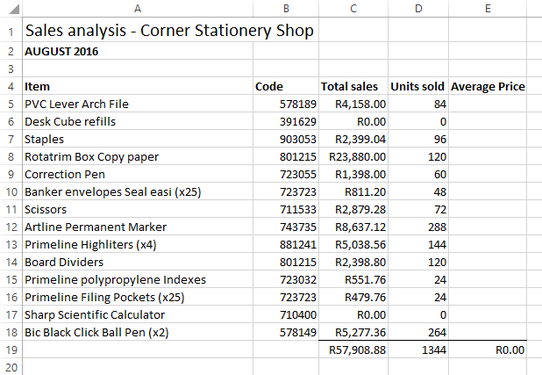 The shop manager needs to calculate the average price of every item, since not all of the items are sold at the same price throughout the month (with month-end specials running the last week of the month, and discount on bulk purchases for corporate clients etc). He enters a formula into Cell E5 to divide the sales value by the number of units sold: =C5/D5 But when he fills the formula downwards, two errors show up in his table, since there were no sales for Desk Cube refills or Sharp Scientific Calculators. His sum function in Cell E19 returns an error too. 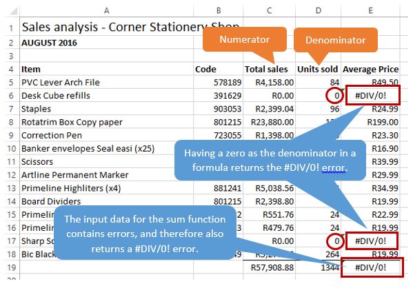 (Please note, summing column E might not be a sensible calculation. Don’t pay too much attention to why the shop manager is calculating this, or what he would use it for. I just need a sum function to illustrate a few things in this example). If you have a short list or a table with only a small number of items (like the one above), you can quite easily deal with these errors by simply clicking one by one to replace the formula with a zero or taking the formula out completely. But if you work with large data sets, this is less than optimal. There is an easier way to keep your tables error-free. The IFERROR formula allows you to decide what you want to do if a calculation returns an error. Do you want to replace it with a zero? Do you prefer to leave it blank? Do want it to show “NONE” OR “N/A”? You can do any of the above. The IFERROR formula is quite simple. Select Cell E6 (the first cell containing an error) and enter the IFERROR formula. The arguments for the formula are as follows: 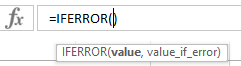 Or if you prefer to make use of the Function Arguments dialog box, click on "fx" to the left of the formula bar (pictured above) to open it up: 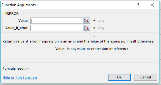 Value The value argument is simply the value that you are trying to calculate - the average price in this example. Therefore, enter the same formula here as previously: C6/D6 Value if error This is where you decide what you want Excel to do with a value if the formula in the value argument returns an error. There are a few options that I can suggest you use to make further calculations easier. To return a zero value, fill in 0 in the second argument. =IFERROR(C6/D6,0) 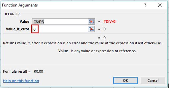 I have entered the formula in the cell containing the error (Cell E6) to show how the function arguments appear, but this formula can be entered in cell E5 and dragged down to copy the same formula down the rest of the column.  To leave the cell blank, enter double quotation marks in the second argument as follows: =IFERROR(C6/D6, "") 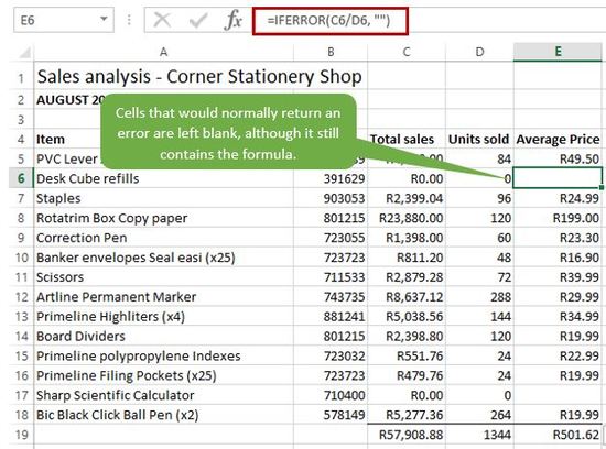 To display some sort of other text description (N/A, or NONE for example) simply enter the description in the second argument in double quotation marks. Note that the sum function in Cell E19 still works if the range you are summing contains text. Formula to enter: =IFERROR(C6/D6, "NONE") 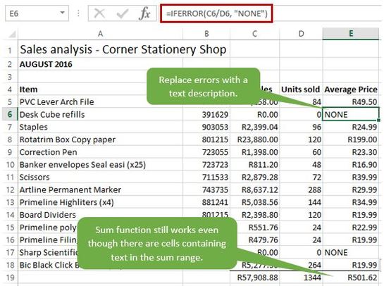 Now you can keep your excel tables neat and error-free. Any other ways that you have used the IFERROR function before? Feel free to share so that others can learn from it too!
0 Comments
Leave a Reply. |
Carine HoughHi, and welcome to my blog :) I am an Excel enthusiast and want to help others keen on improving their own Excel skills. I hope you learn something useful on my blog. 
Categories
All
|
