|
Skills level: Advanced In this lesson, I will illustrate how to use the SUMIF formula. It is a very nifty formula that you can use when you need to sum only certain items according to specific criteria. Imagine for example that you have a fruit cart. You sell Apples, Oranges and Peaches. For every sale that you make, you enter the date of the sale, the type and number of fruits sold, the price per fruit, as well as the total sales neatly into an excel table. At the end of the month, you want to see how much sales you made per fruit, and also how many fruits you have sold of each. 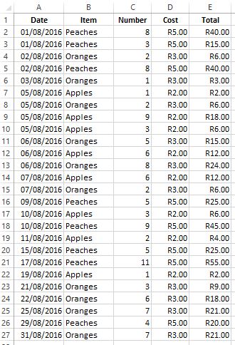 At the end of the month, you want to calculate how many apples, oranges, and peaches you have sold respectively, and how much money you have made with each fruit. Next to my data set, I created a simple table for my totals as follows. 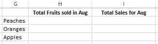 In cell H2, start typing SUMIF and press tab to open the parenthesis. The arguments that are required (also displayed as soon as you pressed tab) is Range, Criteria and Sum Range. 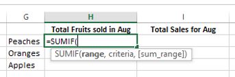 Range The range would be the cells where you want Excel to look for the specific or identifying criteria. In this case, what differentiates your data is the different types of fruit. Therefore, you have to instruct Excel to look in your "Item" column for the specific fruits that you want to count. In this example, you would then choose the range B2:B27. Criteria Next, you need to specify the condition that defines which cells need to be totaled. You need to sum the data that relates to peaches only. You can therefore either add "Peaches", (including the quotation marks as follows: =SUMIF(B2:B27, "Peaches", [sum_range])) in this argument, or (the easier option), simply select cell G2, which already contains the text "Peaches", and would instruct Excel to look for all the rows in which the text (Peaches) has been entered into. Sum_Range Lastly, you need to select the actual sells to sum. We need to add the number of peaches sold in August; therefore, the cells that need to be summed is contained in column C named "Number". Select range C2:C27 by simply highlighting the range. Close your parenthesis and press enter. Your answer should be 53 peaches. 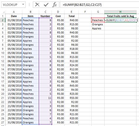 Repeat the same steps to calculate the number of Oranges and Apples sold in Cell H3 and H4. The only argument that would need to be changed is "Criteria". You don't want Excel to search for Peaches this time, but for Oranges (cell G3) and then Apples (cell G4). The "Range" and "Sum_Range" would however be exactly the same, as you are using the same data set to calculate the necessary totals. The formulas for the 3 fruits would look as follows: 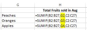 The calculated totals are as follows: 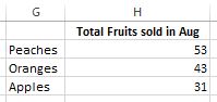 For the more advanced students - You can make both the "Range" and "Sum_Range" absolute references (a shortcut to do this is to press F4 on you keyboard immediately after selecting the appropriate range by highlighting it). Fill downwards to copy the formula for Oranges and Apples. The "Criteria" argument needs to remain relative (without the dollar signs). As you fill down, it has to change to G3 and G4 for it to search for the appropriate text. If you tried the above trick, your formulas should look as follows: 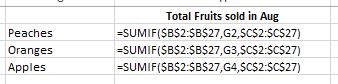 Next we have to calculate the total sales for all the fruits for August, or in other words, how much money did you make with the sale of Peaches, Oranges and Apples respectively. Follow the same method as above. The Sum_Range however, has to be changed to column E in our data set - the Total instead of the Number of fruits. The formula is as follows: =SUMIF(B2:B27,G2,E2:E27) 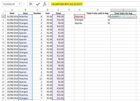 Do the same for Oranges and Apples. If you are feeling brave, try to use the absolute ranges for the first and third argument as follows (do only in Cell I2, and then fill the formula down to I3 and I4). =SUMIF($B$2:$B$27,G2,$E$2:$E$27) =SUMIF($B$2:$B$27,G3,$E$2:$E$27) =SUMIF($B$2:$B$27,G4,$E$2:$E$27) And you're done! Here is your total table. You can finish it off with a simple sum function to see the grand total of fruits sold and your total sales for August. 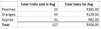 Did you find this post useful? Please share if you think it might help a friend or colleague.
Please feel free to post any questions in the comment section.
2 Comments
MIchael Hough
17/8/2016 23:39:02
Brilliant! Thank you
Elmie
10/9/2016 10:29:15
Love your Website! Leave a Reply. |
Carine HoughHi, and welcome to my blog :) I am an Excel enthusiast and want to help others keen on improving their own Excel skills. I hope you learn something useful on my blog. 
Categories
All
|
