|
Skills Level: Intermediate The IF function in Excel must be one of the most powerful. While it is very simple and easy to understand in its simplest form, the ability to nest functions within the IF function to solve complex problems, makes it extremely useful. Its capability is only limited to its user’s own logical and analytical reasoning ability. The syntax for the simple IF function is as follows: =IF(logical_test, [value_if_true], [value_if_false]) It starts with a logical test which relates simply to a question that you want answered. For e.g., you have a list of exam scores for students. You want to know if students passed or failed. Your IF statement would read something as follows: IF a student achieved 50% or more in the exam, they have passed (therefore the logical test is true, and the formula should return the text “Pass”), else they have failed, in which case the formula should return “Fail” if the exam score is below 50% (and the initial logical test is false). Let’s see how this works practically. Below is the list of students and their exam results. The logical test would be, “Is the exam result larger than or equal to 0.5?”. If it is true, then the formula must return “Pass”, if it is NOT true, then it must return “Fail”. =IF(B2>=0.5, "Pass", "Fail") 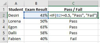 Each argument in the formula can be either a value, a text string, another formula (see nesting IF formulas later) or a combination of all. For example, suppose you deliver the newspaper in your neighbourhood. Not everyone is signed up to receive the newspaper. You therefore have a list of all their names, and a Yes / No column of who wants to receive the newspaper. To easily sum the number of newspapers, you may want to insert an IF formula to return the number 1 if “Yes” is specified in the column or 0 if “No” is indicated. =IF(B3="Yes", 1, 0) 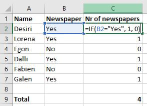 In this way, whenever you convince someone in your list to sign up, you can simply change his choice from “No” to “Yes”, and your total newspapers will automatically change to account for the additional “Yes”. Here is another example. Suppose you have quarterly budget and actual figures for your team. For your meeting, you need to determine who is over, or under budget. Your logical test would be, “Is the Actual figures larger than the Budget figures? If so, then return “Over budget”, if not, then return “Under Budget”. 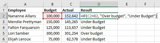 Nested IF function Sometimes, the answer to your question is not a simple yes or no, or over or under budget. Suppose that at the end of the year, employees are awarded a simple KPI score out of 3. One is “Poor”, two is “Average”, and three is “Excellent”. So how can an IF function return 1 of 3 possible results? The answer is by “nesting” the IF function. Nesting simply means, using another formula within a formula. In this case, we will nest a second IF function within an IF function. Let’s see how that works. Your logical reasoning should read something as follows: IF the KPI score is 1, then the outcome is “Poor”, if not 1, then IF (this is your second or “nested” IF) the KPI Score is 2, then outcome is “Average”, and if also not 2, then “Excellent” (which is the last available option if the KPI score is neither 1 or 2, then it must be 3). =IF(B2=1,"Poor",IF(B2=2,"Average","Excellent")) Logical Test 1, Value if true, Value if false is replaced by another IF function to make a further test, Logical Test 2, Value if second test is true, Value if false (both logical test 1 and 2 are false). 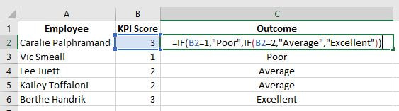 Let’s try a more complex nested IF example. Suppose that sales employees can earn commission based on their sales according to the following scale: 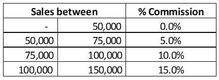 There are 4 possible outcomes, therefore you need 3 IF statements, and the 4th outcome is returned if none of the previous ones are true. =IF(B8<$B$2, $D$2, IF(B8<$B$3, $D$3, IF(B8<$B$4, $D$4, $D$5))) 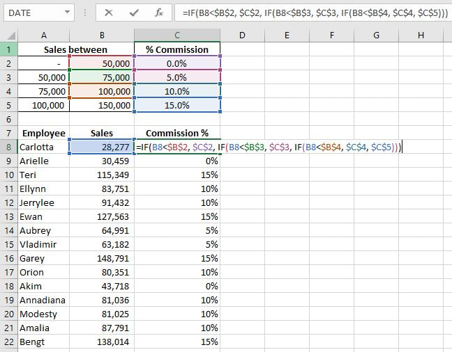 NOTE that Excel evaluates all of the possible outcomes from left to right in your formula. It is therefore important that you think carefully which is the easiest way to reason through your solution. In the above example, we start by asking, is the sales value LESS than R 50 000. If YES then there is only 1 solution, i.e. 0% commission. If not is it LESS than 75 000? The next available solution (5% commission), applies and so on… Consider the first sales amount of R28 277. It is BOTH less than R75 000 and R 50 000. So which commission value does Excel use? 0% or 5%? The answer is simply, the first argument that is true. It is therefore important that you consider the order in which you insert the logical tests in your nested if formula. If you start by reasoning the other way around by saying, “Is the sales amount LARGER than R50 000”, there is MORE THAN ONE result. It can either be 5%, 10%, or 15%, depending on HOW MUCH MORE than R50 000 the sales amount is. Excel will need further instructions (i.e. more formulas) to know how to evaluate the test further to provide 1 result. Therefore, always start with a logical test that will return only 1 result. It will make your life easier, and save you a lot of time. It is possible to nest up to 64 IF functions. That doesn’t mean that you should. Even nesting just a few IF functions gets complicated and difficult to manage and maintain. For example, a nested IF formula written to return one of 7 possible tax brackets (see table below) for different levels of income would look something like this: =IF(B15>$A$12,$C$12,IF(B15>$A$11,$C$11,IF(B15>$A$10,$C$10,IF(B15>$A$9,$C$9,IF(B15>$A$8,$C$8,IF(B15>$A$7,$C$7,$C$6)))))) 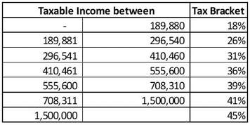 The above formula nests 6 IF functions, imagine a formula containing 64! There are easier ways to go about this. A VLOOKUP formula for example, will do the same thing. The below formula can replace the above nested IF function. =VLOOKUP(B15, $A$6:$C$12, 3) This will be a lesson for another day… IFS function As from the 2016 version of Excel, Microsoft has made things a bit easier for complex IF functions. The IFS function is used when you have multiple IF statements. Instead of having to nest loads of IF functions within each other, the IFS function consists of simple logical test and value-if-true “pairs”. Excel considers each pair in turn. If the logical test is true, it returns the corresponding value, if not, it considers the next logical test in queue, and carries on until the last test and result pair. There is no "or else" or "value-if-false" result if the logical test is NOT true. The formula will return a #N/A error if none of the arguments are true. Its syntax is as follows: =IFS(logical_test1, value_if_true1, …) So you can build a whole list of “If this, then that” scenarios in your formula. Let’s redo the commission exercise to demonstrate how the IFS function will work. Logically the formula would read, “If Sales are less than R 50 000, then 0% commission, If less than R 75 000 then 5%, If less than R 100 000, then 10% and finally if less than R 150 000, then 15%. =IFS(B8<$B$2, $D$2, B8<$B$3, $D$3, B8<$B$4, $D$4, B8<$B$5, $D$5)  Using the function argument box to build your formula will help to see the pairs more clearly. You can build your formula in here if it makes it easier. 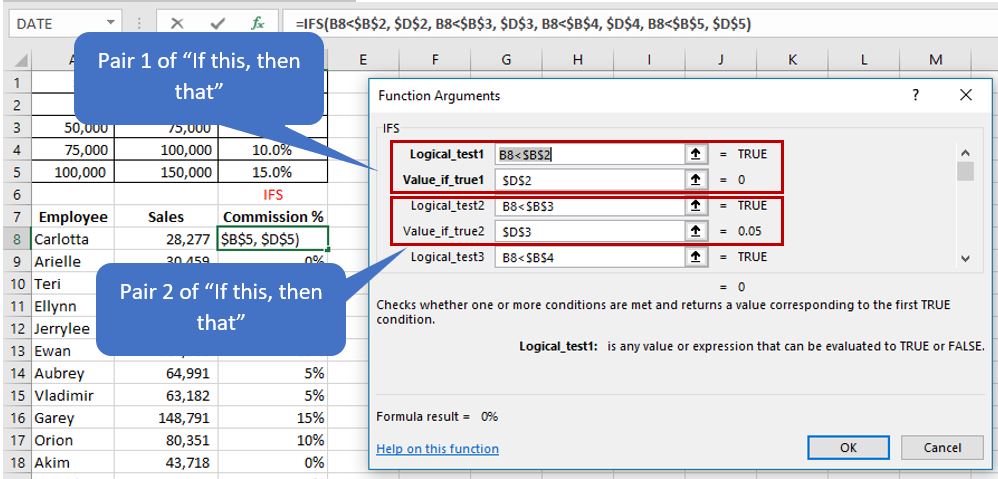 Once again, Excel evaluates each logical test from left to right and returns the result corresponding to the first test that is true, even if subsequent tests will prove to be true as well. (Eg. R 30 459 is both less than R 50 000 and less than R75 000 and less than R 100 000 and less than R150 000. But because the “less than R 50 000” logical test was stated first, it will return the corresponding commission percentage of 0%). You can see this clearly in the argument box. Let’s have a look at Aubrey’s sales of R 64 991. The first test is FALSE (R 64 991 is NOT less than R 50 000), the second test is TRUE (R64 991 is less than R 75 000), the third test is also true (R64 991 is also less than R100 000). But the final result that the formula returns is 5% - the value that corresponds to the FIRST TRUE TEST. 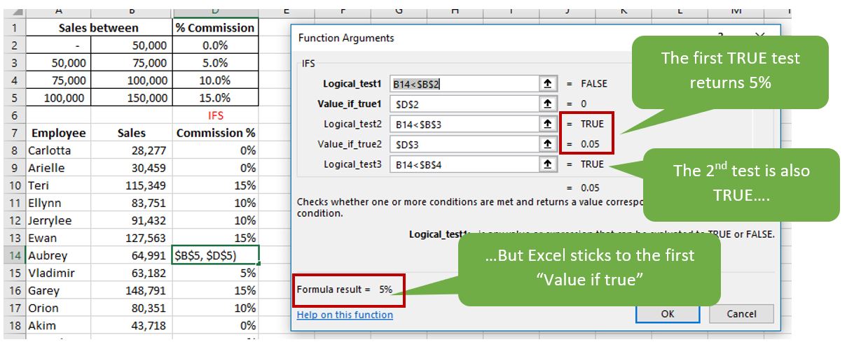 Sometimes, the IFS formula can actually be longer in length than a nested IF, but you will agree that it is easier to reason this way. Excel allows you to include up to 127 logical tests in the IFS formula. Once again, it doesn’t mean that you should. What if you need an "or else" argument. Suppose all kids in the Red, Yellow and Blue class are divided into Team 1, 2 and 3 respectively. There are a few students in the Green, Orange and Purple class that also want to take part but need to be grouped into 1 team (Team 4) because there are not enough kids in each class to make separate teams. Instead of having an argument for all 6 colours, you can simply do 3 arguments for the first 3, and create an "or else" argument at the end as follows. =IFS(A2="Red", 1, A2="Yellow", 2, A2="Blue", 3, TRUE, 4) 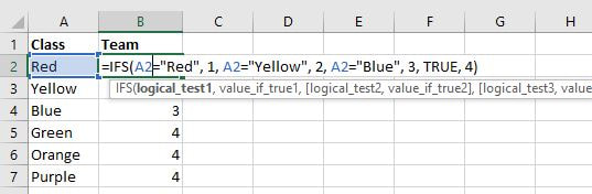 Because you are adding a TRUE logical test and a corresponding value at the end of the formula, if none of the other tests are true, this is the solution that Excel will select, because you have declared the logical test as TRUE (simply by writing “true” as the logical test). See the argument box below to make more sense of this. Since none of the logical tests are true in your formula for the Green class (Because GREEN is not Red, Yellow or Blue), the last remaining logical test to evaluate is the the 4th one that you have inserted as being TRUE, therefore, because the test is true, it’s corresponding value (4 in this case), will be returned. 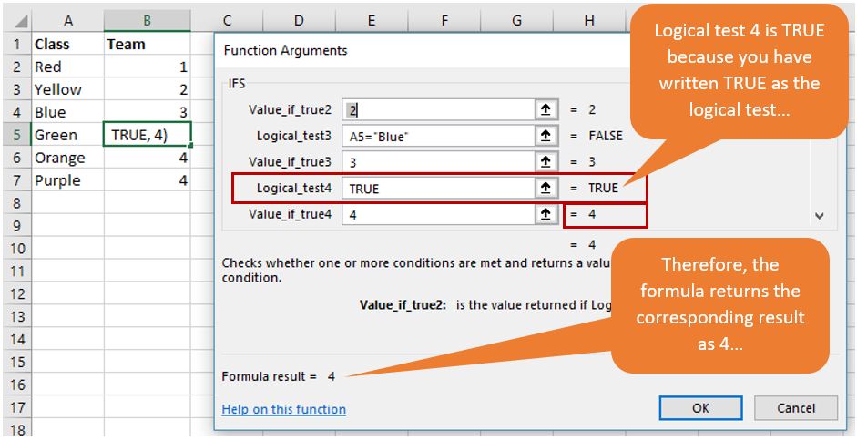 You have therefore essentially created an “or else” or “value if false” argument. Of course you can have your built in “or else” statement return anything you want. Suppose that students in the green, orange or purple class are not to partake in the sport day, you may want the formula to return “Not applicable”. If so, your formula can be adjusted as follows: =IFS(A2="Red", 1, A2="Yellow", 2, A2="Blue", 3, TRUE, "Not applicable") AND & OR Function – Friends of the IF function You will often need to combine AND & OR functions within an IF function. These are very simple functions on their own and quite easy to understand. The AND function returns TRUE if all of its arguments are true. The OR function returns TRUE if either of its arguments are true. Their syntax looks the same. You can include as many logical arguments as you need. =AND(logical1, [logical2],…) =OR(logical1, [logical2],…) Here are a few examples to illustrate: 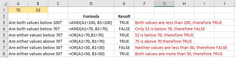 AND function example The AND function is mostly used to find out if a value falls BETWEEN two values. For example, if you get between 45% and 50% for an exam, you are allowed a second opportunity to write an exam in an attempt to pass. To determine whether a list of exam results falls into this category, the AND function can be applied as follows: =AND(A2>=0.45, A2<0.5) 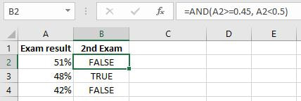 The AND function can be nested within an IF function, to determine “Pass”, “Fail” or “2nd Exam” all in once as follows: =IF(A2>0.5,"Pass",IF(AND(A2>=0.45,A2<0.5),"2nd Exam","Fail")) 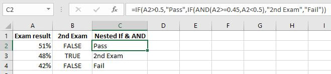 OR function example Suppose employees can earn a bonus if they made more than R100 000 sales OR they have worked more than 48 hours per week. =OR(A2>100000, B2>48) 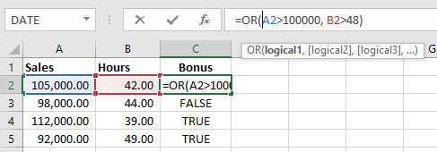 The OR function can be nested in an IF function to return a 10% bonus or leave the cell clear if the requirements for a bonus were not met. =IF(OR(A2>100000, B2>48), 0.1, "") 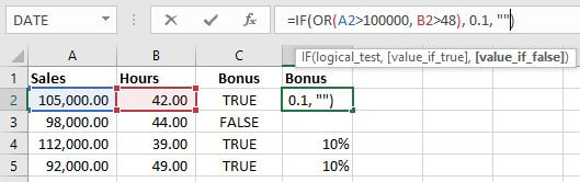 To test what you have learned here, download the challenge below and see how well you can solve the problems. The solution is available for download on the Challenges page.
0 Comments
Leave a Reply. |
Carine HoughHi, and welcome to my blog :) I am an Excel enthusiast and want to help others keen on improving their own Excel skills. I hope you learn something useful on my blog. 
Categories
All
|
||
