|
Skills level: Intermediate Creating a drop-down list in Excel can be a real time-saver. Imagine how much time you waste by typing in the same thing day after day, week after week when you have to complete a list or a register on a regular basis. It might not seem like much at first, but if you add up all the seconds, they add up to minutes, and repeated every week, may amount to a few precious hours over time. There are also consistency benefits that you achieve when making use of drop-down lists, especially if more than one person needs to complete the same register or list. If you had to work with a spreadsheet before where people have used all sorts of different ways to write the same thing, you will know how frustrating it is to clean it up. For example, instead of completing “Monday”, people may have typed “monday”, the abbreviation “Mon” or misspelled it as “Munday”. All these records have a different value, and cannot be summarised in a pivot table for example, since it will be treated as separate records. Creating a list will force people to select the exact value that you need them to, and will not allow them to type their own values, keeping your data neat and clean. I have listed a few questions (imagine doing a survey for example), that all requires a weekday as an answer. This data is in sheet 1 of my workbook. 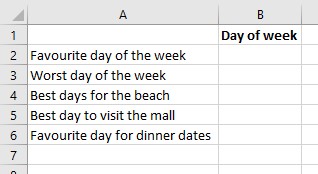 In a separate sheet (Sheet 2), list the days of the week, in the format that you prefer. 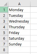 Go back to Sheet 1 and select cell B2. This is the first cell where you would like the drop-down list to appear. Then select Data and Data Validation (in the Data Tools group). Under Validation criteria, select “List” in the “Allow” dropdown box. This basically means that the values that the user is allowed to use is from a predetermined list. Click the button to the right of the “Source” field. Locate your list in Sheet 2. Highlight the list and click enter (or click the same selection button again). Click okay. You will now have a drop-down list in Cell B2.  You will notice that if you type any value other than one from the list, an error will be displayed: 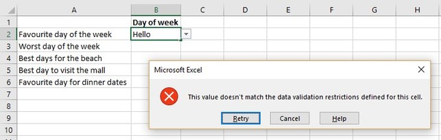 The dropdown list is now only contained in Cell B2. The user will still be able to put any value in the rest of the cells in Column B. To copy the drop-down list to the rest of the cells, you can simply drag the list down the same way you would a formula.  To get rid of a drop-down list, simply follow the same steps as before: Select the Data tab > Data Validation and in the “Allow” dropdown, change the value back to “Any value”. 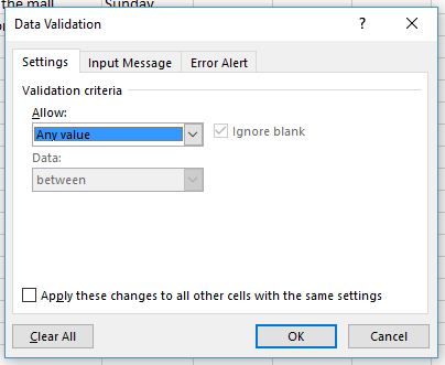
0 Comments
Leave a Reply. |
Carine HoughHi, and welcome to my blog :) I am an Excel enthusiast and want to help others keen on improving their own Excel skills. I hope you learn something useful on my blog. 
Categories
All
|
