|
Skills level: Intermediate
Errors in spreadsheets can be quite annoying. Especially if it is actually not a mistake, but just as a result of the data input. One of the errors that I often come across is the #DIV/0! error when trying to divide by zero. Sometimes, when you export some or other report, it is inevitable that some of the lines will have zero values, which may result in errors when trying to perform certain calculations. You might want to take the errors out, especially if you need the result for further calculations. If you need to sum the calculated column of values for example, the result will also result in an error. Below is a sales report for the Corner Stationery Shop for the month of August. The report includes all the items available to customers (even if none were sold during the month), the total sales value, and the number of items sold in the period.
0 Comments
Skill level: Advanced One of the more exciting features of Excel, is its ability to create interactive charts - charts that change instantly as you change the criteria. Not only is it very impressive and makes you look like an expert, it is actually very easy to set up. Just to give you an idea what an interactive chart would look like, see the chart below. By selecting the relevant department, the chart changes to show only the turnover data for the selected department. 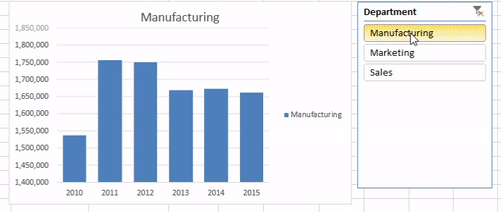 (Don't pay too much attention to the figures, it might not make a lot of sense - I just used random data to generate the chart).
So here’s how to create an interactive pivot chart with the use of a slicer. I have put together a simple data table with 3 columns for Date, Turnover and Department. There are 3 departments and the turnover data stretches over 6 years. Skills level: Intermediate We often need to use the same formula to calculate the same thing for a whole list of items. You may be familiar with the click & drag function that allows you to quickly fill (or copy) the same formula downwards, while Excel assumes that for each subsequent cell into which the formula is copied, the subsequent set of data needs to be used for the calculation. Let’s use an example to illustrate. Below is a simple shopping list, with columns for items, quantity and price per unit. 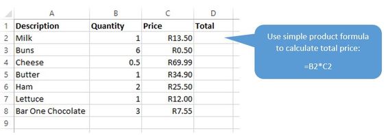 Relative References
To calculate the total cost of your shopping list, you can easily use the product function, or simply enter a multiplication formula into Cell D2 (I am going to use the second formula throughout this example, but the principle will apply to both… or any other formula for that matter): =PRODUCT(B2,C2) OR =B2*C2 Skills level: Intermediate Sometimes, when working with very large spreadsheets, you find yourself navigating back and forth from left to right trying to see all the data on your worksheet. It is quite a nuisance when you have a spreadsheet that has so many columns that does not fit all on your screen. But you also don’t want to delete the columns, because you might want to use the data in the other columns another time. Below is a list of client data. Initially, you only see data completed up to column M. 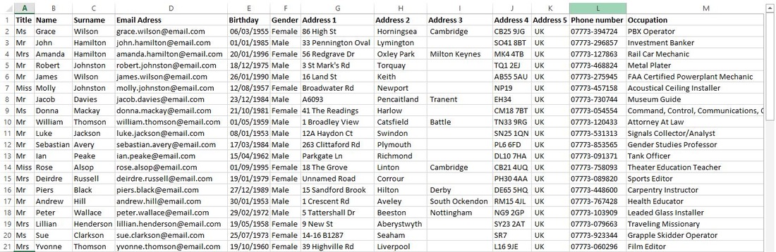 But if you scroll further to the right, there are more columns after Column M with more data. 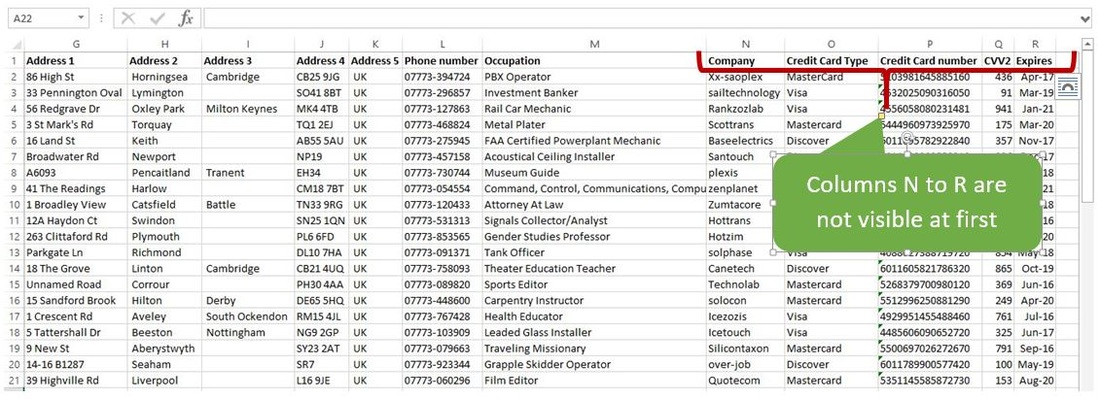 Skills level: Beginner Have you ever wondered why dates are sometimes displayed as a random number? Usually (these days) it starts with a number four, and would be 5 numbers in total. 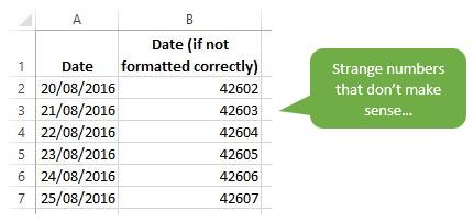 It almost seems like dates are coded in some way. If you thought that, you are absolutely correct. Each and every date has a unique whole number assigned to it, called serial numbers. If you look at the image above, you will see that the numbers follow each other. 20 Aug 2016 is shown as number 42602 (if not formatted correctly as a date), the following day is 42603 and so on.
This property allows you to be able to perform calculations with dates in excel. Because a date is equal to a whole number, you can subtract dates from each other. For example, you may want to know how many days there are between the 20th of August and the 3rd of October - maybe your holiday starts then and you want to start counting down the days! Skills level: Advanced In this lesson, I will illustrate how to use the SUMIF formula. It is a very nifty formula that you can use when you need to sum only certain items according to specific criteria. Imagine for example that you have a fruit cart. You sell Apples, Oranges and Peaches. For every sale that you make, you enter the date of the sale, the type and number of fruits sold, the price per fruit, as well as the total sales neatly into an excel table. At the end of the month, you want to see how much sales you made per fruit, and also how many fruits you have sold of each. 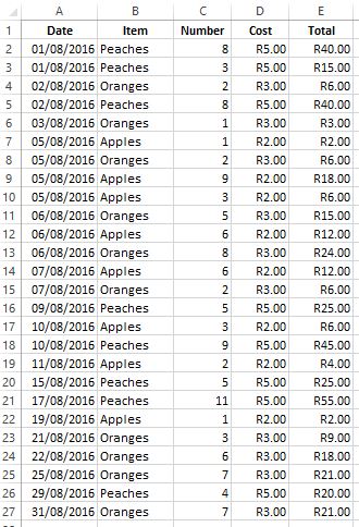 At the end of the month, you want to calculate how many apples, oranges, and peaches you have sold respectively, and how much money you have made with each fruit.
Next to my data set, I created a simple table for my totals as follows. |
Carine HoughHi, and welcome to my blog :) I am an Excel enthusiast and want to help others keen on improving their own Excel skills. I hope you learn something useful on my blog. 
Categories
All
|
